Artemis II Solar Eclipse#
The Artemis II mission recently completed its landmark voyage around the Moon, marking the first departure of humans from Earth orbit in over fifty years. Soon after Artemis II set the record of human distance from Earth, the astronauts took stunning photos of the the solar eclipse they observed on April 6 (EDT) / April 7 (UTC). We highly recommend watching the recording of the eclipse on YouTube; the reactions and descriptions of the astronauts are worth it.
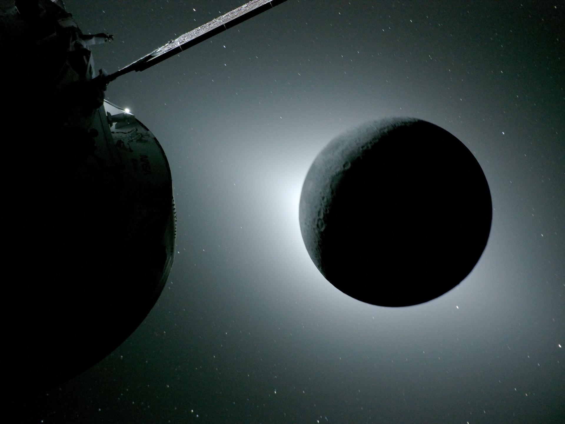
Image credit NASA#
On the SunPy blog, we rarely miss the opportunity to talk about a solar eclipse. So when we saw the eclipse photos taken by the astronauts, we immediately wanted to use SunPy to compare them to other images of the solar corona. Here is one of the amazing photos that has been shared:
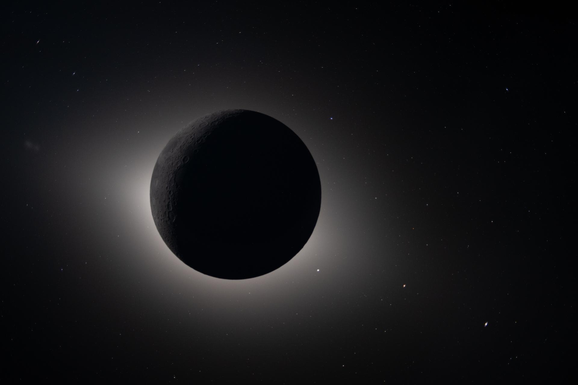
Image credit NASA#
This photo is particularly well suited to comparison with other solar observations because the limb of the Moon is clearly visible, and there are stars and planets in the image we can use as references. Understanding the coordinate system of the photo will allow us to overlay images taken by solar observatories.
The following images in this post, and the code to generate them, are from these two examples in the SunPy gallery:
Visualize the path of Artemis II#
We can use JPL Horizons to obtain the trajectory of Artemis II and to confirm the time range of the solar eclipse.
The sunpy/astropy coordinates framework enables visualizing the trajectory in any desired coordinate frame, and our example shows it in the frame co-rotating with the Moon’s orbit around the Earth.

Visualization of the Artemis II trajectory with the eclipse highlighted.#
Also in our example, we confirm that the total eclipse started around 00:34 UTC and ended around 01:29 UTC.
Determine the coordinate system of the photo#
To be able to compare this image with other observations of the Sun, we need to identify where the camera was pointed and how it was oriented. To do this we perform the following steps:
Extract the time information from the metadata stored in the image.
Use the time information to look up the exact position of Artemis II.
Fit the edge of the Moon to identify the center of the Moon, and the size of the Moon in the image.
Use the three planets visible in the lower right of the image to determine the rotation angle.
Use the planets to fit the distortion of the lens.
The following is an abridged version of the code in our example.
Find the position of Artemis II#
The first step is to know the time the image is taken; we can extract this from the EXIF metadata. As with the trajectory above, we use JPL Horizons to obtain the position of Artemis II at a specific time.
from sunpy.coordinates import get_horizons_coord

artemis2_coord = get_horizons_coord("Artemis II" , "2026-04-07 01:06:19")
Locate the Moon#
The next step is to use a known location in the image as a reference point. The easiest one for us to use is the center of the Moon, which we find by doing edge detection and Hough filtering, using scikit-image.
import numpy as np

from skimage.feature import canny, peak_local_max
from skimage.transform import hough_circle, hough_circle_peaks

edges = canny(eclipse_image, sigma=2)

h, w = eclipse_image.shape
radii = np.arange(0.25*h, 0.4*h, 10)

hough_res = hough_circle(edges, radii)
accums, cx, cy, rad = hough_circle_peaks(hough_res, radii, total_num_peaks=1)

A cropped view of the Moon, showing the results of the canny edge detection algorithm and the Hough filter.#
Calculate the image scale#
Based on the determined center of the Moon and its radius in the image we can construct an initial coordinate system for the image.
from astropy.coordinates import SkyCoord
import astropy.units as u

moon = SkyCoord(coords["moon"], observer=coords["artemis_ii"])
R_moon = 0.2725076 *  u.R_earth  # IAU mean radius
dist_moon = SkyCoord(coords["artemis_ii"]).separation_3d(moon)

moon_angular_width = np.arcsin(R_moon / dist_moon).to(u.arcsec)
im_radius = rad * u.pix
plate_scale = moon_angular_width / im_radius
We can now construct a sunpy Map using this information and overplot the anticipated location of the planets:

Initial coordinate system fit to image, notice that the locations of the highlighted planets are incorrect.#
Determine the camera orientation#
It’s clear from the previous image that we still need to correct for the camera orientation. Having the camera at a specific orientation is tricky even when using a tripod on the Earth’s surface, and we imagine is even trickier when flying through space! Fortunately, the planets serve as excellent reference points.
We determine the camera orientation by using a peak finding algorithm to locate the planets in the image and comparing these positions to the planets coordinates extracted from JPL Horizons.
Doing this gives a \(-21.2^\circ\) roll angle which we can add to our Map metadata.

Image showing the expected positions of the planets and the detected (peaks) positions of the planets, from which the roll angle is calculated.#
Account for lens distortion#
The final correction to apply to our fitted coordinate system is the distortion of the camera lens (a Nikkor AF 135mm f/2D DC). This makes objects distant from the center of the image appear even more distant than they should. We can quantify exactly how much the image has been distorted by comparing the expected versus actual positions of Mars and Mercury (not Saturn as it is too close to the center of the image). We add this distortion to our coordinate system and our planets now appear in the correct place.

Coordinate system fit with additional correction for lens distortion.#
Overplotting Coronagraph Images#
Now that we have established the coordinate system for the eclipse photo, we can compare this observation of the corona to other data. To do this we are going to use the coronagraph (the LASCO instrument) on the Solar and Heliospheric Observatory (SOHO) which is located around the Sun-Earth L1 point. We reproject (or re-grid) these images to the fitted coordinate system of the Artemis II image to compensate for differences in satellite location and point of view, and then crop them to the limb of the moon.

The Artemis II solar eclipse photo with the positions of Mercury, Mars and Saturn highlighted, and coronagraph images from SOHO’s LASCO instrument plotted over the disc of the Moon.#
The coronal structure visible in the LASCO image is not visible in the Artemis II eclipse photo, but the former has undergone significant image processing, and the latter is mostly straight out of the camera. A more scientific comparison may be possible when additional imagery from Artemis II is released in the future.
Closing thoughts#
We think this post is a striking demonstration of what sunpy makes possible.
By combining image metadata, spacecraft ephemerides, and coordinate-aware reprojection, we can place the astronauts’ eclipse photo and SOHO/LASCO coronagraph data into the same physical frame and compare views of the same corona from two very different vantage points.
As a reminder, you can find the full code behind this post in these two examples in the SunPy gallery: Artemis II trajectory and Artemis-II Solar Eclipse.
If you are lucky enough to observe the total solar eclipse which will be visible from parts of Europe on August 12, 2026, remember you can try this type of analysis with your own photos by following our previous blog post!